Theory
The following provides an introduction to the theoretical foundation of the
solver emg3d. More specific theory is covered in the docstrings of many
functions, have a look at the Other functions-section or follow the links to the
corresponding functions here within the theory. If you just want to use the
solver, but do not care much about the internal functionality, then the
function emg3d.solver.solve() is the only function you will ever need. It
is the main entry point, and it takes care whether multigrid is used as a
solver or as a preconditioner (or not at all), while the actual multigrid
solver is emg3d.solver.multigrid().
Note
This section is not an independent piece of work. Most things are taken from one of the following sources:
- [Muld06], pages 634-639:
- The Maxwell’s equations and Discretisation sections correspond with some adjustemens and additions to pages 634-636.
- The start of The Multigrid Method corresponds roughly to page 637.
- Pages 638 and 639 are in parts reproduced in the code-docstrings of the corresponding functions.
- [BrHM00]: This book is an excellent introduction to multigrid methods. Particularly the Iterative Solvers section is taken to a big extent from the book.
Please consult these original resources for more details, and refer to them for citation purposes and not to this manual. More in-depth information can also be found in, e.g., [Hack85] and [Wess91].
Maxwell’s equations
Maxwell’s equations in the presence of a current source \(\mathbf{J}_\mathrm{s}\) are
where the conduction current \(\mathbf{J}_\mathrm{c}\) obeys Ohm’s law,
Here, \(\sigma(\mathbf{x})\) is the conductivity. \(\mathbf{E}(\mathbf{x}, t)\) is the electric field and \(\mathbf{H}(\mathbf{x}, t)\) is the magnetic field. The electric displacement \(\mathbf{D}(\mathbf{x}, t) = \varepsilon(\mathbf{x})\mathbf{E}(\mathbf{x}, t)\) and the magnetic induction \(\mathbf{B}(\mathbf{x}, t) = \mu(\mathbf{x})\mathbf{H}(\mathbf{x}, t)\). The dielectric constant or permittivity \(\varepsilon\) can be expressed as \(\varepsilon = \varepsilon_r \varepsilon_0\), where \(\varepsilon_r\) is the relative permittivity and \(\varepsilon_0\) is the vacuum value. Similarly, the magnetic permeability \(\mu\) can be written as \(\mu = \mu_r\mu_0\), where \(\mu_r\) is the relative permeability and \(\mu_0\) is the vacuum value.
The magnetic field can be eliminated from Equation (1), yielding the second-order parabolic system of equations,
To transform from the time domain to the frequency domain, we substitute
and use a similar representation for \(\mathbf{H}(\mathbf{x}, t)\). The resulting system of equations is
where \(s = -\mathrm{i}\omega\). The multigrid method converges in the
case of the diffusive approximation (with its smoothing and approximation
properties), but not in the high-frequency range (at least not in the
implemented form of the multigrid method in emg3d). The code emg3d
assumes therefore the diffusive approximation, hence only low frequencies are
considered that obey \(|\omega\varepsilon| \ll \sigma\). In this case we
can set \(\varepsilon=0\), and Equation (5) simplifies to
From here on, the hats are omitted. We use the perfectly electrically conducting boundary
where \(\mathbf{n}\) is the outward normal on the boundary of the domain.
The Maxwell’s equations and Ohm’s law are solved in the frequency domain. The time-domain solution can be obtained by taking the inverse Fourier transform.
Note
[Muld06] uses the time convention \(e^{-\mathrm{i}\omega t}\), see Equation (4), with \(s=-\mathrm{i}\omega\). However, the code emg3d uses the convention \(e^{\mathrm{i}\omega t}\), hence \(s=\mathrm{i}\omega\). This is the same convention as used in empymod, and commonly in CSEM.
Laplace domain
It is also possible to solve the problem in the Laplace domain, by
using a real value for \(s\) in Equation (6), instead of the
complex value \(-\mathrm{i}\omega\). This simplifies the problem from
complex numbers to real numbers, which accelerates the computation. It also
improves the convergence rate, as the solution is a smoother function. The
solver emg3d.solver.solve() is agnostic to the data type of the provided
source field, and can solve for real and complex problems, hence frequency and
Laplace domain. See the documentation of the functions
emg3d.fields.get_source_field() and emg3d.models.Model() to see how
you can use emg3d for Laplace-domain computations.
Discretisation
Equation (6) can be discretised by the finite-integration technique ([Weil77], [ClWe01]). This scheme can be viewed as a finite-volume generalization of [Yee66]’s scheme for tensor-product Cartesian grids with variable grid spacings. An error analysis for the constant-coefficient case ([MoSu94]) showed that both the electric and magnetic field components have second-order accuracy.
Consider a tensor-product Cartesian grid with nodes at positions \((x_k, y_l, z_m)\), where \(k=0, \dots, N_x, l=0, \dots, N_y\) and \(m=0, \dots, N_z\). There are \(N_x\times N_y\times N_z\) cells having these nodes as vertices. The cell centres are located at
The material properties, \(\sigma\) and \(\mu_\mathrm{r}\), are assumed to be given as cell-averaged values. The electric field components are positioned at the edges of the cells, as shown in Figure 5, in a manner similar to Yee’s scheme. The first component of the electric field \(E_{1, k+1/2, l, m}\) should approximate the average of \(E_1(x, y_l, z_m)\) over the edge from \(x_k\) to \(x_{k+1}\) at given \(y_l\) and \(z_m\). Here, the average is defined as the line integral divided by the length of the integration interval. The other components, \(E_{2, k, l+1/2, m}\) and \(E_{3, k, l, m+1/2}\), are defined in a similar way. Note that these averages may also be interpreted as point values at the midpoint of edges:
The averages and point-values are the same within second-order accuracy.
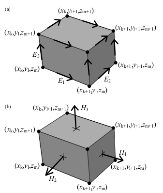
Figure 5: (a) A grid cell with grid nodes and edge-averaged components of the electric field. (b) The face-averaged magnetic field components that are obtained by taking the curl of the electric field.
For the discretisation of the term \(-s\mu_0\sigma\mathbf{E}\) related to Ohm’s law, dual volumes related to edges are introduced. For a given edge, the dual volume is a quarter of the total volume of the four adjacent cells. An example for \(E_1\) is shown in Figure 6(b). The vertices of the dual cell are located at the midpoints of the cell faces.
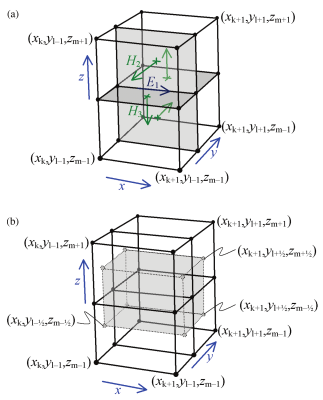
Figure 6: The first electric field component \(E_{1,k,l,m}\) is located at the intersection of the four cells shown in (a). Four faces of its dual volume are sketched in (b). The first component of the curl of the magnetic field should coincide with the edge on which \(E_1\) is located. The four vectors that contribute to this curl are shown in (a). They are defined as normals to the four faces in (a). Before computing their curl, these vectors are interpreted as tangential components at the faces of the dual volume shown in (b). The curl is evaluated by taking the path integral over a rectangle of the dual volume that is obtained for constant x and by averaging over the interval \([x_k,x_{k+1}]\).
The volume of a normal cell is defined as
where
For an edge parallel to the x-axis on which \(E_{1, k+1/2, l, m}\) is located, the dual volume is
With the definitions,
we obtain
Note that Equation (13) does not define \(d_k^x\), etc., at the boundaries. We may simply take \(d^x_0 = h^x_{1/2}\) at \(k = 0\), \(d^x_{N_x} = h^x_{N_x-1/2}\) at \(k = N_x\) and so on, or use half of these values as was done by [MoSu94].
The discrete form of the term \(-s\mu_0\sigma\mathbf{E}\) in Equation (6), with each component multiplied by the corresponding dual volume, becomes \(\mathcal{S}_{k+1/2, l, m}\ E_{1, k+1/2, l, m}\), \(\mathcal{S}_{k, l+1/2, m}\ E_{2, k, l+1/2, m}\) and \(\mathcal{S}_{k, l, m+1/2}\ E_{3, k, l, m+1/2}\) for the first, second and third components, respectively. Here \(\mathcal{S} = -s\mu_0\sigma V\) is defined in terms of cell-averages. At the edges parallel to the x-axis, an averaging procedure similar to (12) gives
\(\mathcal{S}_{k, l+1/2, m}\) and \(\mathcal{S}_{k, l, m+1/2}\) are defined in a similar way.
The curl of \(\mathbf{E}\) follows from path integrals around the edges that bound a face of a cell, drawn in Figure 5(a). After division by the area of the faces, the result is a face-averaged value that can be positioned at the centre of the face, as sketched in Figure 5(b). If this result is divided by \(\mathrm{i}\omega\mu\), the component of the magnetic field that is normal to the face is obtained. In order to find the curl of the magnetic field, the magnetic field components that are normal to faces are interpreted as tangential components at the faces of the dual volumes. For \(E_1\), this is shown in Figure 6. For the first component of Equation (6) on the edge \((k+1/2, l, m)\) connecting \((x_k, y_l, z_m)\) and \((x_{k+1}, y_l, z_m)\), the corresponding dual volume comprises the set \([x_k, x_{k+1}] \times [y_{l-1/2}, y_{l+1/2}] \times [z_{m-1/2}, z_{m+1/2}]\) having volume \(V_{k+1/2,l,m}\).
The scaling by \(\mu_r^{-1}\) at the face requires another averaging step because the material properties are assumed to be given as cell-averaged values. We define \(\mathcal{M} = V\mu_r^{-1}\), so
for a given cell \((k+1/2, l+1/2, m+1/2)\). An averaging step in, for instance, the z-direction gives
at the face \((k+1/2, l+1/2, m)\) between the cells \((k+1/2, l+1/2, m-1/2)\) and \((k+1/2, l+1/2, m+1/2)\).
Starting with \(\mathbf{v}=\nabla \times \mathbf{E}\), we have
Here,
Next, we let
Note that these components are related to the magnetic field components by
where
The discrete representation of the source term \(\mathrm{i}\omega\mu_0\mathbf{J}_\mathrm{s}\), multiplied by the appropriate dual volume, is
Let the residual for an arbitrary electric field that is not necessarily a solution to the problem be defined as
Its discretisation is
The weighting of the differences in \(u_1\), etc., may appear strange. The reason is that the differences have been multiplied by the local dual volume. As already mentioned, the dual volume for \(E_{1,k,l,m}\) is shown in Figure 6(b).
For further details of the discretisation see [Muld06] or [Yee66]. The actual
meshing is done using discretize (part of the
SimPEG-framework). The coordinate system of
discretize uses a coordinate system were positive z is upwards.
The method is implemented in a matrix-free manner: the large sparse linear matrix that describes the discretised problem is never explicitly formed, only its action is evaluated on the latest estimate of the solution, thereby reducing storage requirements.
Iterative Solvers
The multigrid method is an iterative (or relaxation) method and shares as such the underlying idea of iterative solvers. We want to solve the linear equation system
where \(A\) is the \(n\times n\) system matrix and \(x\) the unknown. If \(v\) is an approximation to \(x\), then we can define two important measures. One is the error \(e\)
which magnitude can be measured by any standard vector norm, for instance the maximum norm and the Euclidean or 2-norm defined respectively, by
However, as the solution is not known the error cannot be computed either.
The second important measure, however, is a computable measure, the residual
\(r\) (computed in emg3d.solver.residual())
Using Equation (27) we can rewrite Equation (26) as
from which we obtain with Equation (28) the Residual Equation
The Residual Correction is given by
The Multigrid Method
Note
If you have never heard of multigrid methods before you might want to read through the Multi-what?-section.
Multigrid is a numerical technique for solving large, often sparse, systems of equations, using several grids at the same time. An elementary introduction can be found in [BrHM00]. The motivation for this approach follows from the observation that it is fairly easy to determine the local, short-range behaviour of the solution, but more difficult to find its global, long-range components. The local behaviour is characterized by oscillatory or rough components of the solution. The slowly varying smooth components can be accurately represented on a coarser grid with fewer points. On coarser grids, some of the smooth components become oscillatory and again can be easily determined.
The following constituents are required to carry out multigrid. First, a
sequence of grids is needed. If the finest grid on which the solution is to be
found has a constant grid spacing \(h\), then it is natural to define
coarser grids with spacings of \(2h\), \(4h\), etc. Let the problem on
the finest grid be defined by \(A^h \mathbf{x}^h = \mathbf{b}^h\). The
residual is \(\mathbf{r}^h = \mathbf{b}^h - A^h \mathbf{x}^h\) (see the
corresponding function emg3d.solver.residual(), and for more details
also the function emg3d.core.amat_x()). To find the oscillatory
components for this problem, a smoother or relaxation scheme is applied. Such a
scheme is usually based on an approximation of \(A^h\) that is easy to
invert. After one or more smoothing steps (see the corresponding function
emg3d.solver.smoothing()), say \(\nu_1\) in total, convergence will
slow down because it is generally difficult to find the smooth, long-range
components of the solution. At this point, the problem is mapped to a coarser
grid, using a restriction operator \(\tilde{I}^{2h}_h\) (see the
corresponding function emg3d.solver.restriction(), and for more details,
the functions emg3d.core.restrict_weights() and
emg3d.core.restrict(). On the coarse-grid, \(\mathbf{b}^{2h} =
\tilde{I}^{2h}_h\mathbf{r}^h\). The problem \(\mathbf{r}^{2h} =
\mathbf{b}^{2h} - A^{2h} \mathbf{x}^{2h} = 0\) is now solved for
\(\mathbf{x}^{2h}\), either by a direct method if the number of points is
sufficiently small or by recursively applying multigrid. The resulting
approximate solution needs to be interpolated back to the fine grid and added
to the solution. An interpolation operator \(I^h_{2h}\), usually called
prolongation in the context of multigrid, is used to update \(\mathbf{x}^h
:= \mathbf{x}^h + I^h_{2h}\mathbf{x}^{2h}\) (see the corresponding function
emg3d.solver.prolongation()). Here \(I^h_{2h}\mathbf{x}^{2h}\) is
called the coarse-grid correction. After prolongation, \(\nu_2\) additional
smoothing steps can be applied. This constitutes one multigrid iteration.
So far, we have not specified the coarse-grid operator \(A^{2h}\). It can be formed by using the same discretisation scheme as that applied on the fine grid. Another popular choice, \(A^{2h} = \tilde{I}^{2h}_h A^h I^h_{2h}\), has not been considered here. Note that the tilde is used to distinguish restriction of the residual from operations on the solution, because these act on elements of different function spaces.
If multigrid is applied recursively, a strategy is required for moving through the various grids. The simplest approach is the V-cycle shown in Figure 7 for the case of four grids. Here, the same number of pre- and post-smoothing steps is used on each grid, except perhaps on the coarsest. In many cases, the V-cycle does not solve the coarse-grid equations sufficiently well. The W-cycle, shown in Figure 8, will perform better in that case. In a W-cycle, the number of coarse-grid corrections is doubled on subsequent coarser grids, starting with one coarse-grid correction on the finest grid. Because of its cost, it is often replaced by the F-cycle (Figure 9). In the F-cycle, the number of coarse-grid corrections increases by one on each subsequent coarser grid.
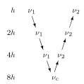
Figure 7: V-cycle with \(\nu_1\) pre-smoothing steps and \(\nu_2\) post-smoothing steps. On the coarsest grid, \(\nu_c\) smoothing steps are applied or an exact solver is used. The finest grid has a grid spacing \(h\) and the coarsest \(8h\). A single coarse-grid correction is computed for all grids but the coarsest.
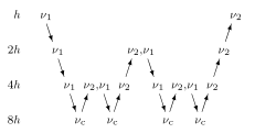
Figure 8: W-cycle with \(\nu_1\) pre-smoothing steps and \(\nu_2\) post-smoothing steps. On each grid except the coarsest, the number of coarse-grid corrections is twice that of the underlying finer grid.
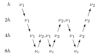
Figure 9: F-cycle with \(\nu_1\) pre-smoothing steps and \(\nu_2\) post-smoothing steps. On each grid except the coarsest, the number of coarse-grid corrections increases by one compared to the underlying finer grid.
One reason why multigrid methods may fail to reach convergence is strong anisotropy in the coefficients of the governing partial differential equation or severely stretched grids (which has the same effect as anisotropy). In that case, more sophisticated smoothers or coarsening strategies may be required. Two strategies are currently implemented, semicoarsening and line relaxation, which can be used on their own or combined. Semicoarsening is when the grid is only coarsened in some directions. Line relaxation is when in some directions the whole gridlines of values are found simultaneously. If slow convergence is caused by just a few components of the solution, a Krylov subspace method can be used to remove them. In this way, multigrid is accelerated by a Krylov method. Alternatively, multigrid might be viewed as a preconditioner for a Krylov method.
Gauss-Seidel
The smoother implemented in emg3d is a Gauss-Seidel smoother. The
Gauss-Seidel method solves the linear equation system \(A \mathbf{x} =
\mathbf{b}\) iteratively using the following method:
where \(L_*\) is the lower triangular component, and \(U\) the strictly upper triangular component, \(A = L_* + U\). On the coarsest grid it acts as direct solver, whereas on the finer grid it acts as a smoother with only few iterations.
See the function emg3d.solver.smoothing(), and for more details, the
functions emg3d.core.gauss_seidel(),
emg3d.core.gauss_seidel_x(), emg3d.core.gauss_seidel_y(),
emg3d.core.gauss_seidel_z(), and also
emg3d.core.blocks_to_amat().
Choleski factorisation
The actual solver of the system \(A\mathbf{x}=\mathbf{b}\) is a
non-standard Cholesky factorisation without pivoting for a symmetric, complex
matrix \(A\) tailored to the problem of the multigrid solver, using only
the main diagonal and five lower off-diagonals of the banded matrix \(A\).
The result is the same as simply using, e.g., numpy.linalg.solve(), but
faster for the particular use-case of this code.
See emg3d.core.solve() for more details.