Info, tips & tricks
Coordinate System
The used coordinate system is shown in Figure 5. It is a right-handed system (RHS) with x pointing East, y pointing North, and z pointing upwards. Azimuth \(\theta\) is defined as the anticlockwise rotation from Easting towards Northing, and elevation \(\varphi\) is defined as the anticlockwise rotation from the horizontal plane up.

Fig. 5 Coordinate system used in emg3d: RHS with positive z upwards.
Grid dimension
The multigrid method, as implemented, puts certain restrictions to the grid dimension.
Note
If you use emg3d through the Simulations / High-level usage
(emg3d.simulations.Simulation) with automatic gridding, or use
emg3d.meshes.construct_mesh, then the following is taken care of by
emg3d itself. However, if you define the computational grids yourself, the
following section is important.
You can provide any three-dimensional regular (stretched) grid into emg3d. However, the implemented multigrid technique works with the existing nodes, meaning there are no new nodes created as coarsening is done by combining adjacent cells. The more times the grid dimension can be divided by two the better it is therefore suited for MG. Ideally, the number should be dividable by two a few times and the dimension of the coarsest grid should be 2 or a small, odd number \(p\), for which good sizes can then be computed with \(p\,2^n\). Good grid sizes (in each direction) up to 1024 are
\(2·2^{3, 4, ..., 9}\): 16, 32, 64, 128, 256, 512, 1024,
\(3·2^{3, 4, ..., 8}\): 24, 48, 96, 192, 384, 768,
\(5·2^{3, 4, ..., 7}\): 40, 80, 160, 320, 640,
and preference decreases from top to bottom row. In sequential order: 16, 24,
32, 40, 48, 64, 80, 96, 128, 160, 192, 256, 320, 384, 512, 640, 768, 1024. You
can obtain the good cell number via emg3d.meshes.good_mg_cell_nr.
Source resolution
Take into consideration that emg3d works with volume-averaged cell properties, and that the fields are defined on edges. This means that the minimum size of a general source is at least as big as the cell surrounding it. In other words, the cell size around your source defines your source resolution.
Solver or Preconditioner
The multigrid method can be used as a solver on its own or as a preconditioner
for a Krylov subspace solver such as BiCGSTAB. This can be controlled through
the parameter sslsolver in emg3d.solver.solve. SSL stands here
for the module scipy.sparse.linalg, and other solvers provided by this
module can be used as well.
Using multigrid as a preconditioner for BiCGSTAB together with semicoarsening and line relaxation is the most stable combination, for which it is the default setting. However, it is also the most expensive setting, and often you can obtain faster results by adjusting the combination of solver, semicoarsening, and line relaxation. Which combination is best (fastest) depends to a large extent on the grid stretching, but also on anisotropy and general model complexity. See «Parameter tests» in the gallery for an example how to run some tests on your particular problem.
CPU & RAM
The multigrid method is attractive because it shows optimal scaling for both runtime and memory consumption. In the following are a few notes regarding memory and runtime requirements. If you are interested in helping to improve either have a look at CPU & RAM.
Runtime
An example of a runtime test is shown in Figure 6. The example shows the runtime to solve for a source of 1.0 Hz at the origin of a homogeneous space of 1.0 Ohm.m, where the grid starts at 32 x 32 x 32 (32,768) to 384 x 384 x 384 (56,623,104). (You can find the script in CPU & RAM.)
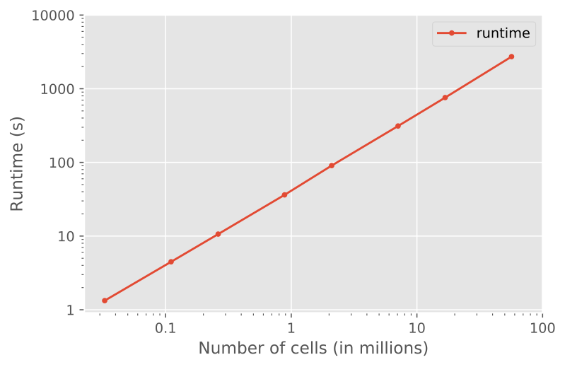
Fig. 6 Runtime as a function of cell size, which shows nicely the linear scaling of multigrid solvers (using a single thread).
The result shows the linear scaling: if you double the number of cells, you double the runtime.
Memory
Most of the memory requirement in emg3d comes from storing the data itself, mainly the fields (source field, electric field, and residual field) and the model parameters (resistivity, eta, mu). For a big model, they some up; e.g., almost 3 GB for an isotropic model with 256 x 256 x 256 cells. The overhead from the computation is small in comparison.
An example of a memory test is shown in Figure 7.
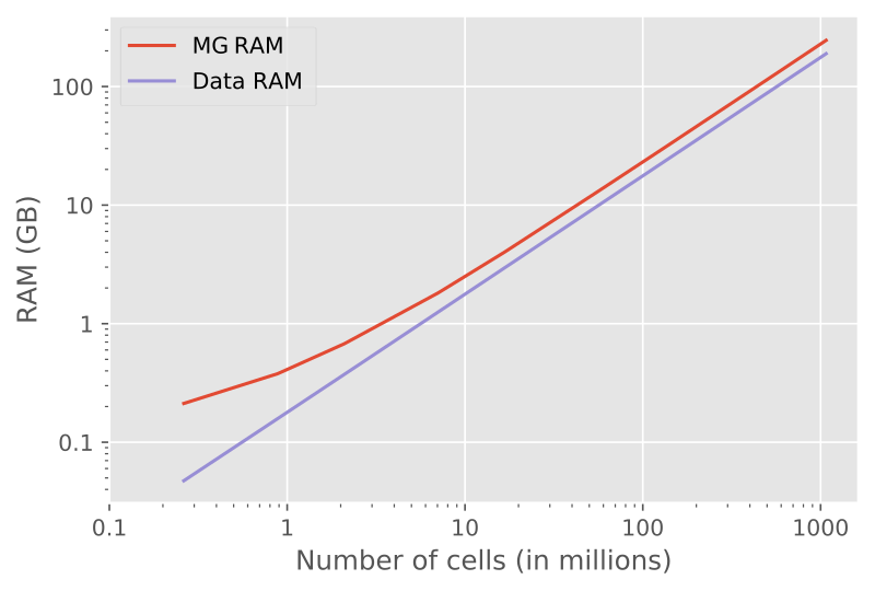
Fig. 7 RAM usage, showing the optimal behaviour of multigrid methods. “Data RAM” is the memory required by the fields (source field, electric field, residual field) and by the model parameters (resistivity; and eta, mu). “MG RAM” is for solving one multigrid F-Cycle.
The results show again nicely the linear behaviour of multigrid; for twice the number of cells twice the memory is required (from a certain size onwards, for small models there is an non-negligible overhead).