construct_mesh
- emg3d.meshes.construct_mesh(frequency, properties, center, domain=None, vector=None, seasurface=None, **kwargs)[source]
Return a TensorMesh for given parameters.
Designing an appropriate grid is the most time-consuming part of any 3D modelling:
Cell sizes should be small enough to represent changes in the model as well as to minimize interpolation errors in the fields.
The computational domain has to be big enough to avoid effects from the boundary condition.
The total number of cells should be small to speed up computation.
These are in itself contradictory requirements, and they additionally depend all on the subsurface properties, the frequency under consideration, and the survey type.
This function is a helper routine to construct an appropriate grid. However, there is no guarantee that it is the best or even a good grid. The constructed grid is frequency- and property-dependent. Some details are explained in other functions:
The minimum cell width \(\Delta_\text{min}\) is a function of
frequency,properties[0],min_width_pps, andmin_width_limits, see Equation (34).The skin depth \(\delta\) is a function of
frequencyandproperties, see Equation (32).The wavelength \(\lambda\) is a function of
frequencyandproperties, see Equation (33).
The relation of the survey domain, computational domain, and buffer zone is shown in Figure 17 for a x-z-section; the y-direction behaves the same as the x-direction (the figures are only visible in the web version of the API docs on https://emg3d.emsig.xyz).
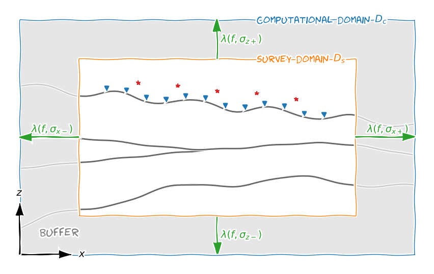
Fig. 17 Relation between survey domain (Ds,
domain), computational domain (Dc), and buffer zone. The survey domain should contain all sources (red stars) and receivers (blue triangles) as well as any important feature that should be represented in the data. The buffer zone is calculated as a function of wavelength with the provided property in the given direction.¶The buffer zone around the survey domain is by default one wavelength. This means that the signal has to travel two wavelengths to get from the end of the survey domain to the end of the computational domain and back. This approach is quite conservative and on the safe side. You can reduce the buffer thickness if you know what you are doing. There are three parameters which influence the thickness of the buffer for a given frequency:
properties, which is used to calculate the skin depth and the wavelength,lambda_factor(default is 1) which sets how many times the wavelength is the thickness of the buffer (relative factor), andmax_buffer, which is an absolute maximum for the buffer thickness. A graphical illustration is given in Figure 18.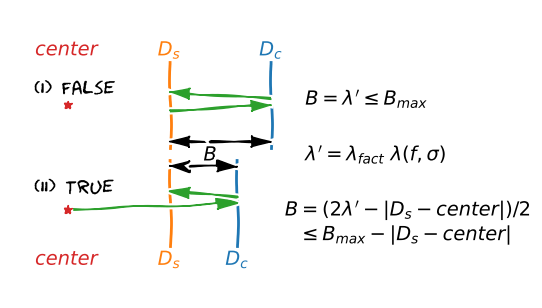
Fig. 18 The thickness of the buffer zone (B) for (I)
lambda_from_center=False(default) and for (II)lambda_from_center=True. Thelambda_factor(\(\lambda_{fact}\)) is a simple scaling factor for the wavelength \(\lambda\). Themax_bufferis an absolute limitation.¶- Parameters
- frequencyfloat
Frequency (Hz) to calculate skin depth; both the minimum cell width and the extent of the buffer zone, and therefore of the computational domain, are a function of skin depth.
- properties{float, array_like}
Properties to calculate the skin depths, which in turn are used to calculate the minimum cell width (usually at source location) and the extent of the buffer around the survey domain. The properties can be either resistivities, conductivities, or the logarithm (natural or base 10) thereof. By default it assumes resistivities, but it can be changed with the parameter
mapping.Five formats are recognized for properties: it can either be a float or a list of 2, 3, 4, or 7 floats. Depending on the format these properties are used to calculate the following parameters:
p: min_width and buffer in all directions;[p1, p2]:p1: min_width,p2: buffer in all directions;
[p1, p2, p3]:p1: min_width,p2: buffer in negative z-direction,p3: buffer in all other directions;
[p1, p2, p3, p4]:p1: min_width,p2: buffer in horizontal directions,p3;p4: buffer in negative; positive z-direction.
[p1, p2, p3, p4, p5, p6, p7]:p1: min_width,p2;p3: buffer in negative; positive x-direction,p4;p5: buffer in negative; positive y-direction,p6;p7: buffer in negative; positive z-direction.
- centerarray_like
Center coordinates (x, y, z). The mesh is centered around this point, which means that here is the smallest cell. Usually this is the source location.
- domain{tuple, list, dict, None}, optional
Contains the survey-domain limits. This domain should include all source and receiver positions as well as any important feature of the model. Format:
([xmin, xmax], [ymin, ymax], [zmin, zmax])or{'x': [xmin, xmax], 'y': [ymin, ymax], 'z': [zmin, zmax]}.It can be None, or individual lists can be None (e.g.,
(None, None,
[zmin, zmax])
), in which case you have to provide either the correspondingdistanceorvector, which is then assumed to span exactly the domain. If only one list is provided it is applied to all dimensions.- distance{tuple, list, dict, None}, optional
An alternative to
domain: Instead of defining the domain in absolute values, they are defined here as distance from the center. Format:([xl, xr], [yl, yr], [zd, zu])or{'x': [xl, xr], 'y': [yl, yr], 'z': [zd, zu]}. From this the domain is given as([cx-xl, cx+xr], [cy-yl, cy+yr], [cz-zd, cz+zu]), wherecenter=(cx, cy, cz).- vector{tuple, ndarray, dict, None}, optional
Contains vectors of mesh-edges that should be used. If provided, the vector must at least include all of the survey domain. If
domainis not provided, it is defined as the minimum/maximum of the provided vector. Format:(xvector, yvector, zvector)or{'x': xvector, 'y': yvector, 'z': zvector}.It can be None, or individual ndarrays can be None (e.g.,
(xvector,
yvector, None)
), in which case you have to provide adomainordistance. If only one ndarray is provided it is applied to all dimensions.- seasurfacefloat, default: None
Air-sea interface. This has only to be set in the marine case, when the mesh in z-direction is sought for (and the interface is not contained in
vector). If set, it will ensure that at the sea surface is an actual boundary. It has to be bigger than the lower limit of the survey domain.- stretching{tuple, list, dict}, default: [1.0, 1.5]
Maximum stretching factors in the form of
[max Ds, max Dc]: the first value is the maximum stretching for the survey domain (default is 1.0), the second value is the maximum stretching for the buffer zone (default is 1.5). If a list is provided the same is used for all three dimension. Alternatively a tuple of three lists can be provided,(x, y, z)or{'x': x, 'y': y, 'z': z}. Note that the first value has no influence on dimensions where avectoris provided.- min_width_limits{float, list, tuple, dict, None}, default: None
Passed through to
cell_widthaslimits. A tuple of three or a dict withx;y;zcan be provided for direction dependent values. Note that this value has no influence on dimensions where avectoris provided.- min_width_pps{float, tuple, dict}, default: 3.0
Passed through to
cell_widthaspps. A tuple of three or a dict withx;y;zcan be provided for direction dependent values. Note that this value has no influence on dimensions where avectoris provided.- lambda_factorfloat, default: 1.0
The buffer is taken as one wavelength from the survey domain. This can be regarded as quite conservative (but safe). The parameter
lambda_factorcan be used to reduce (or increase) this factor.- max_bufferfloat, default: 100_000
Maximum thickness of the buffer zone around survey domain. If
lambda_from_center=True, this is the maximum distance from the center to the end of the computational domain.- lambda_from_centerbool, default: False
Flag how to compute the extent of the computational mesh as a function of wavelength:
False (default): The distance from the edge of the survey domain to the edge of the computational domain is one wavelength.
True: The distance from the center to the edge of the computational domain and back to the end of the survey domain is two wavelengths.
- mapping{str, Map}, default: ‘Resistivity’
Defines what type the input
property_{x;y;z}-values correspond to. By default, they represent resistivities (Ohm.m). The implemented mappings are:'Resistivity'; ρ (Ω m);'Conductivity'; σ (S/m);'LgResistivity'; log_10(ρ);'LgConductivity'; log_10(σ);'LnResistivity'; log_e(ρ);'LnConductivity'; log_e(σ).
- cell_numbersarray_like, optional
List of possible numbers of cells. See
good_mg_cell_nr. Default isgood_mg_cell_nr(1024, 5, 3), which corresponds to numbers 16, 24, 32, 40, 48, 64, 80, 96, 128, 160, 192, 256, 320, 384, 512, 640, 768, 1024.- verbint, default: 0
If 1 verbose, if 0 silent. The info is added either way to the returned mesh as
mesh.construct_mesh_info.
- Returns
- gridTensorMesh
Resulting mesh, a
emg3d.meshes.TensorMeshinstance.