Getting started
There are different usages of emg3d. As an end user you might be interested
in the Simulations / High-level usage: define your survey and your model, and
simulate electromagnetic data for them. As a developer you might be interested
in the Solver-level usage or Command-line interface (CLI-level), to implement emg3d
for instance as a forward modelling kernel in you inversion code. And then
there is also Time-domain modelling.
Here we show first an introductory example of the Simulations / High-level usage. Further down you find an overview and more detailed explanation of the different Usage levels.
Basic Example
The following is a very basic example. To see some more realistic models have
a look at the gallery. First, we
load emg3d, numpy, and matplotlib. Note that this example requires
that you have installed discretize and xarray as well.
In [1]: import emg3d
   ...: import numpy as np
   ...: import matplotlib as mpl
   ...:
One of the elementary ingredients for modelling is a model, in our case a resistivity or conductivity model. emg3d is not a model builder. We just construct here a very simple dummy model. You can see more realistic models in the models section of the gallery.
Grid
We first build a simple four-quadrant grid, centred around the origin.
In [2]: hx = np.ones(2)*5000
   ...: grid = emg3d.TensorMesh(
   ...:         [[5000, 5000], [10000], [5000, 5000]], origin='CCC')
   ...: grid  # QC
   ...:
Out[2]:

  TensorMesh: 4 cells

                      MESH EXTENT             CELL WIDTH      FACTOR
  dir    nC        min           max         min       max      max
  ---   ---  ---------------------------  ------------------  ------
   x      2     -5,000.00      5,000.00  5,000.00  5,000.00    1.00
   y      1     -5,000.00      5,000.00 10,000.00 10,000.00    1.00
   z      2     -5,000.00      5,000.00  5,000.00  5,000.00    1.00
Model
We use the constructed grid to create a simple resistivity model:
In [3]: model = emg3d.Model(
   ...:     grid=grid,
   ...:     property_x=[1, 10, 0.3, 0.3],
   ...:     mapping='Resistivity'
   ...: )
   ...: model  # QC
   ...:
Out[3]: Model: resistivity; isotropic; 2 x 1 x 2 (4)
We defined an isotropic model in terms of resistivities, but through the
mapping parameter one can also define a model in terms of conductivities or
the logarithms thereof.
Quick check how the model looks like:
In [4]: fig, ax = plt.subplots()
   ...: cf = ax.pcolormesh(
   ...:     grid.cell_centers_x/1e3,
   ...:     grid.cell_centers_z/1e3,
   ...:     model.property_x[:, 0, :].T,
   ...:     shading='nearest',
   ...:     norm=mpl.colors.LogNorm(),
   ...: )
   ...: fig.colorbar(cf)
   ...: ax.set_title(r'Depth slice ($\Omega$ m)');
   ...: ax.set_xlabel('Easting (km)');
   ...: ax.set_ylabel('Depth (km)');
   ...:
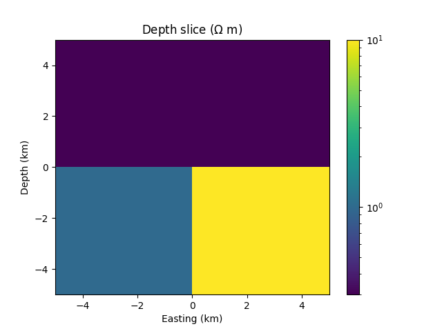
So we have an upper halfspace of 0.3 Ohm.m, a lower-left quadrant of 1 Ohm.m, and a lower-right quadrant of 10 Ohm.m.
Survey
Now that we have a model we need to define our survey. Currently there are three source types implemented,
and two receiver types,
We are going to define a simple survey with an electric dipole source and a line of electric point receivers.
In [5]: source = emg3d.TxElectricDipole(
   ...:     coordinates=(-3000, 0, 0, 0, 0)  # x, y, z, azimuth, elevation
   ...: )
   ...:
   ...: offsets = np.linspace(-2000, 3000, 21)
   ...: receivers = emg3d.surveys.txrx_coordinates_to_dict(
   ...:     emg3d.RxElectricPoint,
   ...:     coordinates=(offsets, 0, 0, 0, 0),  # x, y, z, azimuth, elevation
   ...: )
   ...:
   ...: survey = emg3d.Survey(
   ...:     sources=source,
   ...:     receivers=receivers,
   ...:     frequencies=1.0,       # Hz
   ...: )
   ...:
   ...: survey  # QC
   ...:
Out[5]:
:: Survey ::

<xarray.Dataset>
Dimensions:   (src: 1, rec: 21, freq: 1)
Coordinates:
  * src       (src) <U6 'TxED-1'
  * rec       (rec) <U7 'RxEP-01' 'RxEP-02' 'RxEP-03' ... 'RxEP-20' 'RxEP-21'
  * freq      (freq) <U3 'f-1'
Data variables:
    observed  (src, rec, freq) complex128 (nan+nanj) (nan+nanj) ... (nan+nanj)
Attributes:
    noise_floor:     None
    relative_error:  None
Simulation
Now that we have a model and a survey we can define our simulation:
In [6]: sim = emg3d.Simulation(
   ...:     survey=survey,
   ...:     model=model,
   ...: )
   ...:
   ...: sim  # QC
   ...:
Out[6]:
:: Simulation ::

- Survey: 1 sources; 21 receivers; 1 frequencies
- Model: resistivity; isotropic; 2 x 1 x 2 (4)
- Gridding: Single grid for all sources and frequencies; 96 x 48 x 64 (294,912)
From the output we see that we defined a survey with one source, 21 receivers, and one frequency. We see that we have a model, defined as resistivity, which consists of four cells. And we see that the simulation created a computational grid of 96x48x64 cells.
A simulation takes many input parameters, and you should really read the API
reference of emg3d.simulations.Simulation. Particularly important are
the gridding parameters, and as such it is highly recommended to also read
emg3d.meshes.construct_mesh. The simulation will try its best to create
suitable computational grids. However, these are not necessarily the best ones,
and the user has to pay attention to the grid creation. Also, the default grids
will most likely be quite big, to be on the safe side. Providing suitable user
inputs can significantly reduce the grid sizes and therefore computational
time!
So lets check in more detail the computational grid it created:
In [7]: comp_model = sim.get_model(source='TxED-1', frequency=1.0)
   ...: comp_model.grid
   ...:
Out[7]:

  TensorMesh: 294,912 cells

                      MESH EXTENT             CELL WIDTH      FACTOR
  dir    nC        min           max         min       max      max
  ---   ---  ---------------------------  ------------------  ------
   x     96     -6,939.37     13,615.81     91.89  3,045.59    1.42
   y     48    -11,286.30     11,286.30     91.89  3,045.59    1.42
   z     64    -13,651.53      2,245.90     91.89  1,866.31    1.21
We can see that the grid extends further in the directions where there are higher resistivities. For instance, in positive z we have 0.3 Ohm.m, so the grid does only extend roughly to +2.2 km. In positive x and z as well as in positive and negative y we have 10 Ohm.m, so the grid goes to over 10 km.
Computing the fields is now a simple command,
In [8]: sim.compute()
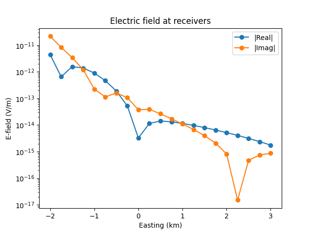
Results
Let’s plot the electric field at receiver locations (the responses):
In [9]: responses = sim.data.synthetic.data.squeeze()
   ...: fig, ax = plt.subplots()
   ...: ax.semilogy(offsets/1e3, abs(responses.real), 'C0o-', label='|Real|')
   ...: ax.semilogy(offsets/1e3, abs(responses.imag), 'C1o-', label='|Imag|')
   ...: ax.legend()
   ...: ax.set_title('Electric field at receivers')
   ...: ax.set_xlabel('Easting (km)')
   ...: ax.set_ylabel('E-field (V/m)')
   ...:
Out[9]: Text(0, 0.5, 'E-field (V/m)')
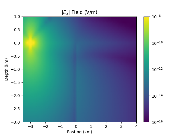
We can also get the entire electric field in a similar way as we got the computational model, and plot it for QC:
In [10]: efield = sim.get_efield(source='TxED-1', frequency=1.0)
   ....:
   ....: fig, ax = plt.subplots()
   ....: cf = ax.pcolormesh(
   ....:     efield.grid.cell_centers_x/1e3,
   ....:     efield.grid.nodes_z/1e3,
   ....:     abs(efield.fx[:, 24, :].T),
   ....:     shading='gouraud',
   ....:     norm=mpl.colors.LogNorm(vmin=1e-16, vmax=1e-8),
   ....: )
   ....: fig.colorbar(cf)
   ....: ax.set_xlim([-3.5, 4])
   ....: ax.set_ylim([-3, 1])
   ....: ax.set_title(r'|$E_x$| Field (V/m)');
   ....: ax.set_xlabel('Easting (km)');
   ....: ax.set_ylabel('Depth (km)');
   ....:
This is frankly a very fast rundown, and many things are only scratched at the surface or not explained at all. However, you should find much more information and explanation in the rest of the manual, and many examples in the gallery.
Usage levels
Simulations / High-level usage

Fig. 1 Workflow for the high-level usage: A Simulation needs a Model and a Survey. A survey contains all acquisition parameters such as sources, receivers, frequencies, and data, if available. A model contains the subsurface properties such as conductivities or resistivities, and the grid information.
Simulate responses for electric and magnetic receivers due to electric and magnetic sources, in parallel. If data is provided it can also compute the misfit and the gradient of the misfit function. It includes automatic, source and frequency dependent gridding.
Note: In addition to emg3d this requires the soft dependency xarray
(tqdm and discretize are recommended).
Solver-level usage

Fig. 2 Workflow for the solver-level usage: The solve function requires a
Model A and a Source-Field b. It then solves Ax=b and
returns x, the electric field, corresponding to the provided subsurface
model and source field.
The solver level is the core of emg3d: It solves Maxwell’s equations for the provided subsurface model and the provided source field using the multigrid method, returning the resulting electric field.
The function emg3d.solver.solve_source simplifies the solver scheme. It
takes a model, a source, and a frequency, avoiding the need to generate the
source field manually, as shown in Figure 3.

Fig. 3 Simplified solver-level workflow: The solve_source function requires a
Model, a Source, and a frequency. It generates the source field
internally, and returns x, the electric field, corresponding to the
provided input.
Note: This requires only emg3d (discretize is recommended).
Command-line interface (CLI-level)

Fig. 4 CLI-level usage: file-driven command-line usage of the high-level (Simulation) functionality of emg3d.
The command-line interface is a terminal utility for the high-level (Simulation) usage of emg3d. The model and the survey have to be provided as files (HDF5, npz, or json), various settings can be defined in the config file, and the output will be written to the output file (see also I/O & Persistence).
Note: In addition to emg3d this requires the soft dependency xarray
(tqdm and discretize are recommended), and h5py if the provided
files are in the HDF5 format.
Time-domain modelling
Time-domain modelling with emg3d is possible, but it is not implemented in the
high-level class Simulation. It has to be carried out by using
emg3d.time.Fourier, together with the Solver-level usage mentioned
above. Have a look at the repo https://github.com/emsig/article-TDEM.
Note: In addition to emg3d this requires the soft dependency empymod
(discretize is recommended).